Plot ImageCollection#
The geetools extention contains a set of functions for rendering charts from the results of spatiotemporal reduction of images within an ee.ImageCollection. The choice of function dictates the arrangement of data in the chart, i.e., what defines x- and y-axis values and what defines the series. Use the following function descriptions and examples to determine the best function for your purpose.
Set up environment#
Install all the required libs if necessary and perform the import satements upstream.
# uncomment if installation of libs is necessary
# !pip install earthengine-api geetools
from matplotlib import pyplot as plt
from datetime import datetime as dt

import ee
import geetools #noqa: F401
# uncomment if authetication to GEE is needed
# ee.Authenticate()
# ee.Intialize(project="<your_project>")
Example data#
The following examples rely on a ee.FeatureCollection composed of three ecoregion features that define regions by which to reduce image data. The ImageCollection data loads the modis vegetation indicies and subset the 2010 2020 decade of images.
## Import the example feature collection and drop the data property.
ecoregions = (
    ee.FeatureCollection("projects/google/charts_feature_example")
    .select(["label", "value", "warm"])
)


## Load MODIS vegetation indices data and subset a decade of images.
vegIndices = (
    ee.ImageCollection("MODIS/061/MOD13A1")
    .filter(ee.Filter.date("2010-01-01", "2020-01-01"))
    .select(["NDVI", "EVI"])
)
Plot dates#
The plot_dates* methods will plot the values of the image collection using their dates as x-axis values.
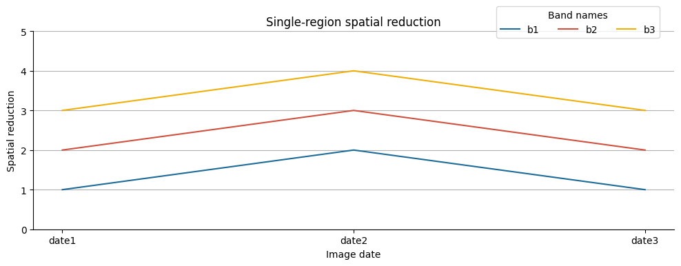
series by bands#
Image date is plotted along the x-axis according to the dateProperty property. Series are defined by image bands. Y-axis values are the reduction of images, by date, for a single region.
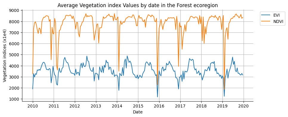
Use plot_series_by_bands to display an image time series for a given region; each image band is presented as a unique series. It is useful for comparing the time series of individual image bands. Here, a MODIS image collection with bands representing NDVI and EVI vegetation indices are plotted. The date of every image observation is included along the x-axis, while the mean reduction of pixels intersecting a forest ecoregion defines the y-axis.
fig, ax = plt.subplots(figsize=(10, 4))
region = ecoregions.filter(ee.Filter.eq("label", "Forest"))
vegIndices.geetools.plot_dates_by_bands(
    region = region.geometry(),
    reducer = "mean",
    scale = 500,
    bands = ["NDVI", "EVI"],
    ax = ax,
    dateProperty = "system:time_start",
)

# once created the axes can be modified as needed using pure matplotlib functions
ax.set_ylabel("Vegetation indices (x1e4)")
ax.set_title("Average Vegetation index Values by date in the Forest ecoregion")

plt.show()
See API
plot_dates_by_bands: Plot the reduced data for each image in the collection by bands on a specific region.datesByBands: Reduce the data for each image in the collection by bands on a specific region.
Plot series by region#
Image date is plotted along the x-axis according to the dateProperty property. Series are defined by regions. Y-axis values are the reduction of images, by date, for a single image band.

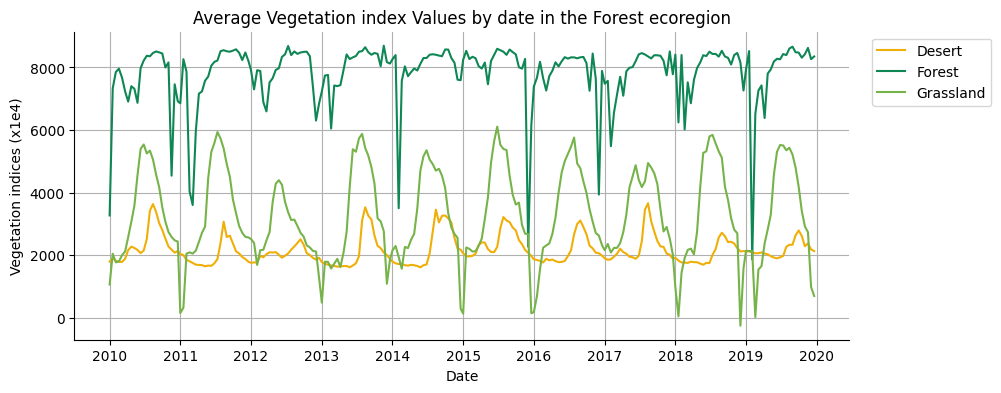
Use plot_dates_by_regions to display a single image band time series for multiple regions; each region is presented as a unique series. It is useful for comparing the time series of a single band among several regions. Here, a MODIS image collection representing an NDVI time series is plotted for three ecoregions. The date of every image observation is included along the x-axis, while mean reduction of pixels intersecting forest, desert, and grasslands ecoregions define y-axis series.
fig, ax = plt.subplots(figsize=(10, 4))
region = ecoregions.filter(ee.Filter.eq("label", "Forest"))
vegIndices.geetools.plot_dates_by_regions(
    band = "NDVI",
    regions = ecoregions,
    label = "label",
    reducer = "mean",
    scale = 500,
    ax = ax,
    dateProperty = "system:time_start",
    colors = ['#f0af07', '#0f8755', '#76b349']
)

# once created the axes can be modified as needed using pure matplotlib functions
ax.set_ylabel("Vegetation indices (x1e4)")
ax.set_title("Average Vegetation index Values by date in the Forest ecoregion")

plt.show()
See API
plot_dates_by_regions: Plot the reduced data for each image in the collection by regions for a single band.datesByRegions: Reduce the data for each image in the collection by regions for a single band.
PLot DOY#
DOY stands for day of year. The plot_doyseries* methods will plot the values of the image collection using the day of year as x-axis values.
Note that .plot_doyseries* functions take two reducers: one for region reduction (regionReducer) and another for intra-annual coincident day-of-year reduction (yearReducer). Examples in the following sections use ee.Reducer.mean() as the argument for both of these parameters.
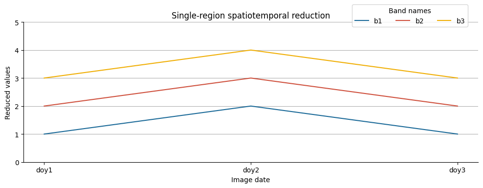
Plot DOY by bands#
Image day-of-year is plotted along the x-axis according to the dateProperty property. Series are defined by image bands. Y-axis values are the reduction of image pixels in a given region, grouped by day-of-year.
Use plot_doy_by_bands to display a day-of-year time series for a given region; each image band is presented as a unique series. It is useful for reducing observations occurring on the same day-of-year, across multiple years, to compare e.g. average annual NDVI and EVI profiles from MODIS, as in this example.
fig, ax = plt.subplots(figsize=(10,4))

vegIndices.geetools.plot_doy_by_bands(
    region = ecoregions.filter(ee.Filter.eq("label", "Grassland")).geometry(),
    spatialReducer = "mean",
    timeReducer = "mean",
    scale = 500,
    bands = ["NDVI", "EVI"],
    ax = ax,
    dateProperty = "system:time_start",
    colors = ['#e37d05', '#1d6b99']
)

# once created the axes can be modified as needed using pure matplotlib functions
ax.set_ylabel("Vegetation indices (x1e4)")
ax.set_title("Average Vegetation index Values by doy in the Grassland ecoregion")

plt.show()
---------------------------------------------------------------------------
KeyboardInterrupt                         Traceback (most recent call last)
Cell In[11], line 3
      1 fig, ax = plt.subplots(figsize=(10,4))
----> 3 vegIndices.geetools.plot_doy_by_bands(
      4     region = ecoregions.filter(ee.Filter.eq("label", "Grassland")).geometry(),
      5     spatialReducer = "mean",
      6     timeReducer = "mean",
      7     scale = 500,
      8     bands = ["NDVI", "EVI"],
      9     ax = ax,
     10     dateProperty = "system:time_start",
     11     colors = ['#e37d05', '#1d6b99']
     12 )
     14 # once created the axes can be modified as needed using pure matplotlib functions
     15 ax.set_ylabel("Vegetation indices (x1e4)")

File ~/checkouts/readthedocs.org/user_builds/geetools/envs/v1.16.0/lib/python3.10/site-packages/geetools/ee_image_collection.py:2168, in ImageCollectionAccessor.plot_doy_by_bands(self, region, spatialReducer, timeReducer, dateProperty, bands, labels, colors, ax, scale, crs, crsTransform, bestEffort, maxPixels, tileScale)
   2106 """Plot the reduced data for each image in the collection by bands on a specific region.
   2107
   2108 This method is plotting the reduced data for each image in the collection by bands on a specific region.
   (...)
   2152         collection.geetools.plot_doy_by_bands(region, "mean", "mean", 10000, "system:time_start")
   2153 """
   2154 # get the reduced data
   2155 raw_data = self.doyByBands(
   2156     region=region,
   2157     spatialReducer=spatialReducer,
   2158     timeReducer=timeReducer,
   2159     dateProperty=dateProperty,
   2160     bands=bands,
   2161     labels=labels,
   2162     scale=scale,
   2163     crs=crs,
   2164     crsTransform=crsTransform,
   2165     bestEffort=bestEffort,
   2166     maxPixels=maxPixels,
   2167     tileScale=tileScale,
-> 2168 ).getInfo()
   2170 # transform all the dates strings into int object and reorder the dictionary
   2171 def to_int(d):

File ~/checkouts/readthedocs.org/user_builds/geetools/envs/v1.16.0/lib/python3.10/site-packages/ee/computedobject.py:107, in ComputedObject.getInfo(self)
    101 def getInfo(self) -> Optional[Any]:
    102   """Fetch and return information about this object.
    103
    104   Returns:
    105     The object can evaluate to anything.
    106   """
--> 107   return data.computeValue(self)

File ~/checkouts/readthedocs.org/user_builds/geetools/envs/v1.16.0/lib/python3.10/site-packages/ee/data.py:1128, in computeValue(obj)
   1125 body = {'expression': serializer.encode(obj, for_cloud_api=True)}
   1126 _maybe_populate_workload_tag(body)
-> 1128 return _execute_cloud_call(
   1129     _get_cloud_projects()
   1130     .value()
   1131     .compute(body=body, project=_get_projects_path(), prettyPrint=False)
   1132 )['result']

File ~/checkouts/readthedocs.org/user_builds/geetools/envs/v1.16.0/lib/python3.10/site-packages/ee/data.py:408, in _execute_cloud_call(call, num_retries)
    406 num_retries = _max_retries if num_retries is None else num_retries
    407 try:
--> 408   return call.execute(num_retries=num_retries)
    409 except googleapiclient.errors.HttpError as e:
    410   raise _translate_cloud_exception(e)

File ~/checkouts/readthedocs.org/user_builds/geetools/envs/v1.16.0/lib/python3.10/site-packages/googleapiclient/_helpers.py:130, in positional.<locals>.positional_decorator.<locals>.positional_wrapper(*args, **kwargs)
    128     elif positional_parameters_enforcement == POSITIONAL_WARNING:
    129         logger.warning(message)
--> 130 return wrapped(*args, **kwargs)

File ~/checkouts/readthedocs.org/user_builds/geetools/envs/v1.16.0/lib/python3.10/site-packages/googleapiclient/http.py:923, in HttpRequest.execute(self, http, num_retries)
    920     self.headers["content-length"] = str(len(self.body))
    922 # Handle retries for server-side errors.
--> 923 resp, content = _retry_request(
    924     http,
    925     num_retries,
    926     "request",
    927     self._sleep,
    928     self._rand,
    929     str(self.uri),
    930     method=str(self.method),
    931     body=self.body,
    932     headers=self.headers,
    933 )
    935 for callback in self.response_callbacks:
    936     callback(resp)

File ~/checkouts/readthedocs.org/user_builds/geetools/envs/v1.16.0/lib/python3.10/site-packages/googleapiclient/http.py:191, in _retry_request(http, num_retries, req_type, sleep, rand, uri, method, *args, **kwargs)
    189 try:
    190     exception = None
--> 191     resp, content = http.request(uri, method, *args, **kwargs)
    192 # Retry on SSL errors and socket timeout errors.
    193 except _ssl_SSLError as ssl_error:

File ~/checkouts/readthedocs.org/user_builds/geetools/envs/v1.16.0/lib/python3.10/site-packages/google_auth_httplib2.py:218, in AuthorizedHttp.request(self, uri, method, body, headers, redirections, connection_type, **kwargs)
    215     body_stream_position = body.tell()
    217 # Make the request.
--> 218 response, content = self.http.request(
    219     uri,
    220     method,
    221     body=body,
    222     headers=request_headers,
    223     redirections=redirections,
    224     connection_type=connection_type,
    225     **kwargs
    226 )
    228 # If the response indicated that the credentials needed to be
    229 # refreshed, then refresh the credentials and re-attempt the
    230 # request.
    231 # A stored token may expire between the time it is retrieved and
    232 # the time the request is made, so we may need to try twice.
    233 if (
    234     response.status in self._refresh_status_codes
    235     and _credential_refresh_attempt < self._max_refresh_attempts
    236 ):

File ~/checkouts/readthedocs.org/user_builds/geetools/envs/v1.16.0/lib/python3.10/site-packages/httplib2/__init__.py:1724, in Http.request(self, uri, method, body, headers, redirections, connection_type)
   1722             content = b""
   1723         else:
-> 1724             (response, content) = self._request(
   1725                 conn, authority, uri, request_uri, method, body, headers, redirections, cachekey,
   1726             )
   1727 except Exception as e:
   1728     is_timeout = isinstance(e, socket.timeout)

File ~/checkouts/readthedocs.org/user_builds/geetools/envs/v1.16.0/lib/python3.10/site-packages/httplib2/__init__.py:1444, in Http._request(self, conn, host, absolute_uri, request_uri, method, body, headers, redirections, cachekey)
   1441 if auth:
   1442     auth.request(method, request_uri, headers, body)
-> 1444 (response, content) = self._conn_request(conn, request_uri, method, body, headers)
   1446 if auth:
   1447     if auth.response(response, body):

File ~/checkouts/readthedocs.org/user_builds/geetools/envs/v1.16.0/lib/python3.10/site-packages/httplib2/__init__.py:1396, in Http._conn_request(self, conn, request_uri, method, body, headers)
   1394     pass
   1395 try:
-> 1396     response = conn.getresponse()
   1397 except (http.client.BadStatusLine, http.client.ResponseNotReady):
   1398     # If we get a BadStatusLine on the first try then that means
   1399     # the connection just went stale, so retry regardless of the
   1400     # number of RETRIES set.
   1401     if not seen_bad_status_line and i == 1:

File ~/.asdf/installs/python/3.10.17/lib/python3.10/http/client.py:1375, in HTTPConnection.getresponse(self)
   1373 try:
   1374     try:
-> 1375         response.begin()
   1376     except ConnectionError:
   1377         self.close()

File ~/.asdf/installs/python/3.10.17/lib/python3.10/http/client.py:318, in HTTPResponse.begin(self)
    316 # read until we get a non-100 response
    317 while True:
--> 318     version, status, reason = self._read_status()
    319     if status != CONTINUE:
    320         break

File ~/.asdf/installs/python/3.10.17/lib/python3.10/http/client.py:279, in HTTPResponse._read_status(self)
    278 def _read_status(self):
--> 279     line = str(self.fp.readline(_MAXLINE + 1), "iso-8859-1")
    280     if len(line) > _MAXLINE:
    281         raise LineTooLong("status line")

File ~/.asdf/installs/python/3.10.17/lib/python3.10/socket.py:717, in SocketIO.readinto(self, b)
    715 while True:
    716     try:
--> 717         return self._sock.recv_into(b)
    718     except timeout:
    719         self._timeout_occurred = True

File ~/.asdf/installs/python/3.10.17/lib/python3.10/ssl.py:1307, in SSLSocket.recv_into(self, buffer, nbytes, flags)
   1303     if flags != 0:
   1304         raise ValueError(
   1305           "non-zero flags not allowed in calls to recv_into() on %s" %
   1306           self.__class__)
-> 1307     return self.read(nbytes, buffer)
   1308 else:
   1309     return super().recv_into(buffer, nbytes, flags)

File ~/.asdf/installs/python/3.10.17/lib/python3.10/ssl.py:1163, in SSLSocket.read(self, len, buffer)
   1161 try:
   1162     if buffer is not None:
-> 1163         return self._sslobj.read(len, buffer)
   1164     else:
   1165         return self._sslobj.read(len)

KeyboardInterrupt:
See API
plot_doy_by_bands: Plot the reduced data for each image in the collection by bands on a specific region.doyByBands: Aggregate the images that occurs on the same day and then reduce each band on a single region.
Plot doy by regions#
Image day-of-year is plotted along the x-axis according to the dateProperty property. Series are defined by regions. Y-axis values are the reduction of image pixels in a given region, grouped by day-of-year, for a selected image band.
Use plot_doy_by_regions to display a single image band day-of-year time series for multiple regions, where each distinct region is presented as a unique series. It is useful for comparing annual single-band time series among regions. For instance, in this example, annual MODIS-derived NDVI profiles for forest, desert, and grassland ecoregions are plotted, providing a convenient comparison of NDVI response by region. Note that intra-annual observations occurring on the same day-of-year are reduced by their mean.
fig, ax = plt.subplots(figsize=(10,4))

vegIndices.geetools.plot_doy_by_regions(
    regions = ecoregions,
    label = "label",
    spatialReducer = "mean",
    timeReducer = "mean",
    scale = 500,
    band = "NDVI",
    ax = ax,
    dateProperty = "system:time_start",
    colors = ['#f0af07', '#0f8755', '#76b349']
)

# once created the axes can be modified as needed using pure matplotlib functions
ax.set_ylabel("NDVI (x1e4)")
ax.set_title("Average NDVI Values by doy in each ecoregion")

plt.show()
See API
plot_doy_by_regions: Plot the reduced data for each image in the collection by regions for a single band.doyByRegions: Aggregate the images that occurs on the same day and then reduce a single band on multiple regions.
plot doy by year#
Image day-of-year is plotted along the x-axis according to the dateProperty property. Series are defined by years present in the ImageCollection. Y-axis values are the reduction of image pixels in a given region, grouped by day-of-year, for a selected image band.
Use plot_doy_by_years to display a day-of-year time series for a given region and image band, where each distinct year in the image collection is presented as a unique series. It is useful for comparing annual time series among years. For instance, in this example, annual MODIS-derived NDVI profiles for a grassland ecoregion are plotted for years 2012 and 2019, providing convenient year-over-year interpretation.
# reduce the regions to grassland
grassland = ecoregions.filter(ee.Filter.eq("label", "Grassland"))

# for plot speed and lisibility only keep 2 years (2010 and 2020) for the example
indices = vegIndices.filter(
        ee.Filter.Or(
            ee.Filter.date("2012-01-01", "2012-12-31"),
            ee.Filter.date("2019-01-01", "2019-12-31"),
        )
)
fig, ax = plt.subplots(figsize=(10,4))

indices.geetools.plot_doy_by_years(
    band = "NDVI",
    region = grassland.geometry(),
    reducer = "mean",
    scale = 500,
    ax = ax,
    colors = ['#39a8a7', '#9c4f97']
)

# once created the axes can be modified as needed using pure matplotlib functions
ax.set_ylabel("NDVI (x1e4)")
ax.set_title("Average NDVI Values by day of year for Grassland")

plt.show()
See API
plot_doy_by_years: Plot the reduced data for each image in the collection by years for a single band.doyByYears: Aggregate for each year on a single region a single band.
plot doy by seasons#
In case the observation you want to analyse are only meaningful on a subset of the year a variant of the previous method allows you to plot the data by season. The season is defined by the seasonStart and seasonEnd parameters, which are 2 numbers between 1 and 366 representing the start and end of the season. To set them, the user can use the or time.struct_time method to get the day of the year.
ee.Date("2022-06-01").getRelative("day", "year").getInfo()
dt(2022, 6, 1).timetuple().tm_yday
fig, ax = plt.subplots(figsize=(10,4))

indices.geetools.plot_doy_by_seasons(
    band = "NDVI",
    region = grassland.geometry(),
    seasonStart = ee.Date("2022-04-15").getRelative("day", "year"),
    seasonEnd = ee.Date("2022-09-15").getRelative("day", "year"),
    reducer = "mean",
    scale = 500,
    ax = ax,
    colors = ['#39a8a7', '#9c4f97']
)

# once created the axes can be modified as needed using pure matplotlib functions
ax.set_ylabel("NDVI (x1e4)")
ax.set_title("Average NDVI Values during growing season in Grassland")

plt.show()
See API
plot_doy_by_seasons: Plot the reduced data for each image in the collection by years for a single band.doyBySeasons: Aggregate for each year on a single region a single band.